Quenching an ultracold bosonic gas in a ring across the Bose–Einstein condensation phase transition is known, and has been experimentally observed, to lead to the spontaneous emergence of persistent currents. The present work examines how these phenomena generalize to a system of two experimentally accessible explicitly two-dimensional co-planar rings with a common interface, or to the related lemniscate geometry, and demonstrates an emerging independence of winding numbers across the rings, which can exhibit flow both in the same and in opposite directions. The observed persistence of such findings in the presence of dissipative coupled evolution due to the local character of the domain formation across the phase transition and topological protection of the randomly emerging winding numbers should be within current experimental reach.
Figures5
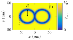
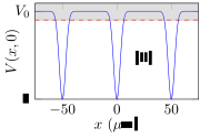
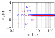
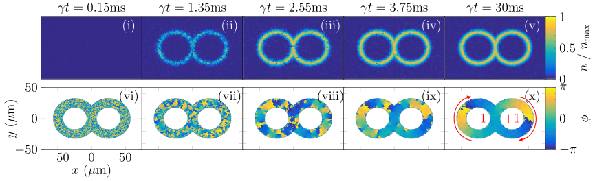
Figure 1.Condensate growth in the double-ring geometry, with ring radius R=25μm, width w=6μm, and the inter-ring shift is δ=0, see equation (5). (a), (i): the double-ring potential, (ii) its cross section along y=0 (blue solid curve) and (iii) the evolution of the winding number over scaled time γt for the left (blue squares) and right (red circles) rings. (b), (i)–(v): the density evolution in scaled time, with nmax=73μm−2. (vi)–(x): the corresponding phase profiles. For clarity, these have been masked by the Heaviside function Θ(0.9V0−Vdr(x,y)), which filter out the contributions falling within the grey shaded area in (a), (ii).
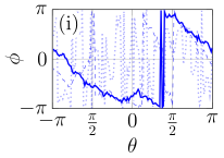
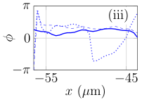
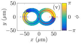
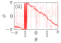
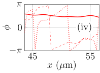
Figure 2.Azimuthal [(i) and (ii)] and radial [(iii) and (iv)] condensate phase shown for times γt=(1.35,3.75,30) ms (dotted, dashed, solid lines respectively, with increasing opacity for later times). The azimuthal phase is extracted around the lines (i) ρ(x+R,y)=R and (ii) ρ(x−R,y)=R, while the radial phase profile is displayed along cross section y=0. (v) References to the azimuthal (solid) and radial (dashed) phase profiles are superimposed on the 2D phase plot. Other parameters are the same as in figure 1.
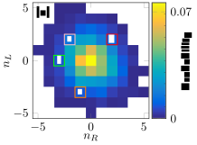
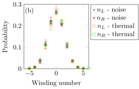
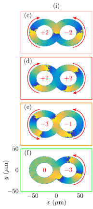
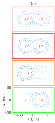
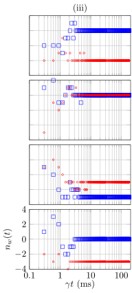
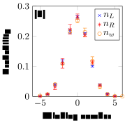
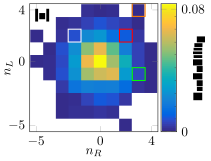
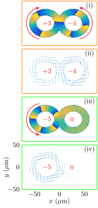
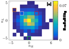
Figure 3.The distribution of persistent currents in the double-ring geometry. (a): the 2D histogram of winding numbers, produced by results of 5000 runs of the SPGPE. Coloured squares correspond to the phase plots and velocity fields below. (b): marginal histogram distributions for the left (nL) and right (nR) rings, comparing growth from noise to instantaneous thermal quench simulations, error bars contain the true probability within a 95% confidence interval. (c)–(f): (i) phase plots, (ii) velocity fields, and (iii) winding number evolutions of a typical single numerical run from within the selected squares from (a). Parameters are the same as figure 1.
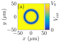
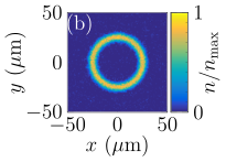
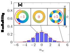
Figure 4.Formation of persistent currents in the single-ring trap. (a) The trapping potential from equation (7) with parameters R=25μm and w=6μm. (b) An equilibrium density profile produced by a single run of the SPGPE. (c) The distribution of winding numbers nw after 5000 realisations of the SPGPE, shown along with a fitted Gaussian distribution (red curve), whose standard deviation is σ=1.5338. Insets show examples of phase profiles for nw=(−1,0,5) from left to right, masked by the Heaviside function Θ(0.9V0−Vsr(x,y)) for clarity. (d) Marginal distributions for the single-ring nw, and for the left (nL) and right (nR) rings from figure 3.
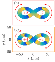
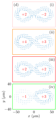
Figure 5.The quench in the 2D Bose gas confined in the lemniscate potential. (a) The 2D histogram of winding numbers produced by 5000 runs of simulations of the SPGPE. Coloured squares correspond to the surrounding phase plots and velocity fields. (b)–(c) Selected phase plots, showing winding-number sets (2,−2) and (4,3). (d) Panels (i)–(iv) display velocity fields of selected squares from (a). Other parameters are the same as in figure 1.
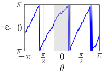
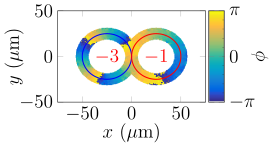
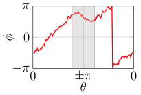
Figure 6.Centre: 2D phase profile for the case (−3,−1). Left: azimuthal phase profile for the left ring, grey highlights the region of overlap between the rings. Right: azimuthal phase for the right ring, shifted in the x-axis such that the overlap region of the two rings occurs in the grey region. Other parameters are the same as in figure 1.
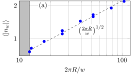
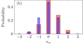
Figure 7.(a) A power-law dependence given by equation (B.1). Each blue point is the measurement of ⟨∣nw∣⟩ after 5000 SPGPE simulations for varying w=(3,6)μm and R=(12.5,18.75,25,37.5,50)μm. The grey region covers the range of R<2w, when there is no central hole in the density. (b) The distribution of observed winding numbers, produced by the thermal quench with ramp time τr=0.025 s. Red (wide) bars are experimental data from Corman et al. for the single ring, based on 36 runs, while blue (thin) bars represent numerical data collected from 5000 realisations of the SPGPE. Parameters are specified in the main text.
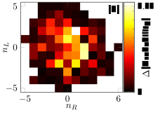
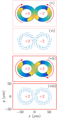
Figure 8.Distribution of persistent currents in a double-ring geometry, with δ=w/2. (a) 2D histogram of observed winding numbers after 5000 runs of the SPGPE. Coloured squares correspond to the surrounding phase plots and velocity fields. (b) Measure of the relative difference between the δ=0 and δ=w/2 histograms. Note the different spatial extent of the colorbar in this case, corresponding to a maximum relative error of 6.3%. (i)–(viii) Phase plots and velocity fields of selected squares from (a). Other parameters are the same as figure 1.
We have explored the spontaneous growth of persistent currents in a
quenched 2D Bose gas in the co-planar side-by-side double-ring geometry.
The emerging persistent currents are stable and long-lived, and do not
transfer between the rings. The overall value of the winding number in each
ring behaves independently, which can be directly attributed to the
importance of the local nature of phase establishment in the azimuthal
direction, an observation that remains valid even when allowing for radial
random phase variations. While the distribution of winding numbers across
the two rings can therefore be directly mapped onto the well-known results
for the single-ring setting, it is important to note that the azimuthal
phase gradient in each ring (for a given non-zero winding number) is not
constant, in direct contrast to the constant phase gradient of the
single-ring case. This is one manifestation of the non-homeomorphism
between a single torus and a 2-torus. Remarkably, however, this is not
necessarily an impediment to potential future atomtronic devices, which
could utilize the observed robust nature of the superfluid current
configuration. The independence of the ring winding numbers and stability
of the formed supercurrents may facilitate a well-controlled current
transfer protocol between rings. Such deterministic transfer of winding
numbers across multiple-loop atomtronic architectures is a promising
direction for future research.
Varying the separation of the rings demonstrates the ability to modify the
atom transfer between the rings and generate vortices between them.
However, there is no sign of angular momentum transfer between the rings.
The robustness of the persistent currents after the quench holds steadfast
even against the change of trap geometry, such as replacement of the double
ring by the lemniscate potential, where one might naively expect
uncorrelated persistent currents in individual rings to be suppressed due
to atomic motion along a “figure-of-eight” path. We also varied the
phenomenological damping parameter γ in a broad range of values, and
extended the simulation time, which produced no evidence of decay,
confirming the efficiency of the topological protection of the
spontaneously generated winding numbers.
A natural question suggested by the present results is the transfer of the
winding numbers between the rings, which will be the subject of further
work. The ability to control the transfer of winding numbers could be
envisaged as a prototypical atomtronic switch, providing an avenue for
controllable realization of coherent quantum phase slips required for the
Mooij-Harmans qubit. A hot topic of current studies of toroidal BECs is the
supercurrent decay mechanism, an understanding of which could help control
the transfer of current states between the rings. The Gross-Pitaevskii
equation and its many extensions do not capture supercurrent decay, even at
finite temperature, without an external barrier. However, due to roughness
of the potential, the decay time for large winding numbers in experiments
is on the order of seconds, whereas nw∼1 may be stable on times on
the order of minutes. Theoretical studies of the decay mechanism so far
have all relied on effects along the annulus, caused by a repulsive
barrier, the decay being visualized as vortices crossing the barrier region
radially. It has been shown that the temperature-induced decay does not fit
the Caldeira-Leggett superconductivity model, i.e. the observed decay rate
does not match simple models of quantum tunnelling and thermal activation
of phase slips. Using a truncated Wigner approximation, some of the
disagreements between theory and experiment have been attributed to thermal
fluctuations; however, exact identification of the decay mechanism remains
an open question.